

How to do an Interworksheet VLOOKUP?
To do an Interworksheet VLOOKUP in Excel follow the steps given below:
1. Write =VLOOKUP(

Now, after writing =VLOOKUP there will be 4 parameters called lookup value, table array, and col-index-num and range lookup
2. Choose LOOKUP value as Employee ID so that it will become =VLOOKUP(B4,

3. Go to Sheet 11

Note – When you go to Sheet 11 you will see that in the Function bar Sheet 11 is written along with an exclamation mark which means that excel should know that in which worksheet table array is sitting
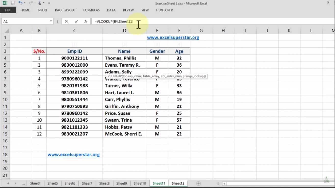
4. Select the table and press F4 so the formula will become =VLOOKUP(B4,Sheet11!$C$3:$F$15,

Note – Immediately press comma after pressing F4
Now col_index_num means you have the chosen 4 table column and now you want the name. So the name is in the 2nd column
5. Write 2 after selecting the col_index_num and the formula will become =VLOOKUP(B4, Sheet11!$C$3:$F$15,2,

Note – Press Comma after writing every function
Now the last parameter will aks us TRUE or FALSE. So FALSE means an exact match. If you are looking for a number and the number is exactly the same then it is FALSE.
6. Write FALSE or 0 and close the bracket so the formula will become =VLOOKUP(B4,Sheet11!$C$3:$F$15,2,0)

7. Press Enter
As you can see how easily I got the answer as Hobbs, Patsy which is the names from the list of Worksheet 12 besides the Employee Id column
8. Now copy-paste the formula to the bottom of the table

Now here you will see that 2 out 4 names are showing N/A. This could possibly due to 2 reasons
1. There is no data which means the Employee ID showing here is having no data in Worksheet 12
2. The number in the cell is formatted as text which means there is an exclamation mark before the Employee ID
9. So go to the exclamation flag and select the option Convert to Number
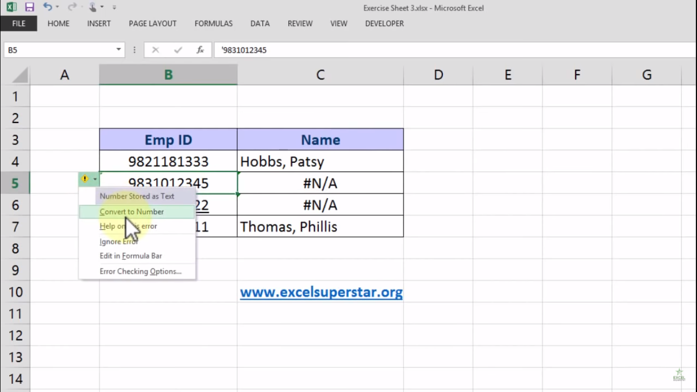
10. After converting to the number you will see the names of the Employees
Note – By chance want to know the age of these Employees then the process is the same so you just have to do follow the step by step process given above
instead of col_index_num which is 2 you write 4 so that the formula will be =VLOOKUP(B4,Sheet11!$C$3:$F$15,4,0) because there are no more than 4 columns in the table

Conclusion:
So from these 3 names, we have completed the Intersheet VLOOKUP in Excel. Also, visit our website excelsuperstar.org to learn more tricks and functions in excel. If you have any doubt while applying this function then do comment below I will be glad to help you out.