
A home is incomplete without its essentials like Furniture, Utensils, and electricity. Similarly, an Excel Spreadsheet is incomplete without its main essential i.e. Excel Tables.
Excel is a spreadsheet that contains a number of rows and columns in the form of a list. The Excel Tables is a feature in Excel which was introduced in the year 2007. These Excel Tables make managing and extending the list easier. Tables were introduced for other office products like Word and PowerPoint but Excel Tables are different and more powerful.
What is an Excel Table?
Excel Table is a powerful and cool feature of Excel that involves managing and analyzing a group of data. A range of cells can be converted into a Table with a blink of an eye. Excel Tables are a great source for creating a Pivot Table.
To create a Pivot Table the raw data must be in Table Format and this can be done by learning to create Excel Tables and its power-packed features. The main reason to learn to use Excel Table is that working with data is easier in Excel Tables.

Don’t be shocked to see from where did this table come in Excel. This short article will help you to know everything about the Excel Tables. First, let us see how to create an Excel Tables in Excel.
How to Create an Excel Table?
Creating an Excel Table is no big task. A task which can be carried out within just a blink of an eye. The time taken to format your data into rows and columns is not included. Once your data is completely ready by removing all the blank rows and columns and assign a unique name for each column.
Steps to Create an Excel Tables:
1. Select any cell in your data range.
2. Press the shortcut key CTRL + T
OR
Go to the Insert Tab > Click on Table. (Create Table Dialog box appears)
3. Check the range and tick on my table contains headers. Press OK.

NOTE: Another shortcut to open the Create Table Dialog box is Ctrl + L
Knowing the Parts of Excel Tables
Let us learn the various elements that are Part of Excel Tables. There are 7 elements the Excel Table comprises of but basically, when you create a table you will see these 4 elements:
1. Column Header: This part of the Excel Table is in the first row in the table. It contains the column heading that gives identification to each column.
NOTE: Column Header must be unique and cannot be blank or contain any formula.
2. The body of the Table: This part of the Excel Table is where all the data and the formula is entered.
3. The row in the Table: The body of the Excel Table contains one or more rows. To differentiate better between the rows, alternate shading is applied.
4. The column in the Table: This part of the Excel Table is a must and it should contain at least one column.

The basic elements of the Excel Tables are now clear. We move forward to the next is the Design Table Tool Tab.
What is the Design Table Tool Tab?
The Design Table Tool Tab is activated when we select any cell inside the Excel Table. Clicking anywhere outside the Excel Table will make this Design Tab to disappear.
This tab contains all the options and the commands which are related to tables. In this Tab, you will be able to change the name of the Table, Resize the table, Change the Table Design, Change the Table Style Option, Enable and Disable the table elements.
NOTE: The Design Table tool Tab is not available in the Excel Online Ribbon

Name an Excel Table
Whenever an Excel Table is created, it gives a default name to the Table starting Table1 and increases in sequence. It is easier to work with the Table Name at a future stage. It is advised to Name an Excel Table with a short name.
It is one of my favorite features as it makes it easy to refer to the table’s data in the formula. But there are certain rules while naming an Excel Table:
1. A maximum of 255 characters can be entered in the Excel Table Name.
2. The Table Name should not contain any space or any other characters in between.
3. The Table Name does not start with a number, it can start with Alphabets or an underscore.
4. Table Name must be unique within a workbook.
Steps to Name an Excel Table:
1. Click on the table to activate the Design Table Tool Tab.
2. Enter the Name in the Table Name option in the Properties Group of the Design Table Tool Tab.
3. Press Enter when you finish entering the name in the Excel Tables Name option.

After naming your Excel Tables there might come a need to change the name of the same Excel Table. You can Rename the Excel Tables and solve the above problem.
Remove Duplicates from the Excel Table
Duplication takes place when records are entered more than once in the spreadsheet. Duplicate records can be seen in more than one column of the data. Removing of duplicates from the range of cells will affect only the selected range and not the entire data.
The steps to remove duplication from the range of cells and from the table are different. Steps to remove duplicates from the table are as follow:
1. Select any cell in the table to activate the Table Tools Option.
2. Click on the Design tab > Tools Group > Remove Duplicates.
3. Put a tick on the column header name from which you want to remove duplicates. Press OK.

You see that all the duplicate values of the column selected are removed and a fresh table is seen in front of you.

NOTE: By default, the entire table is selected when you click on the Remove Duplicates option.
The Layman thing that you would have done to remove duplicates is going through the entire one after another locate the duplicate and then delete them. The removal of duplicates from the table is the same as you remove duplicates from the Data Tab.
Convert an Excel Table back to Normal Range
You changed your mind and now you want to convert the Excel Table into the Normal Range of cells. Well, why do you want to go back to leaving such amazing Excel Table features? I would suggest No, don’t do it but after all, it’s your choice.
Converting to the Normal range of cells is easy and simple with the help of few clicks. Using any of the three ways that suit you best can help you to convert an Excel table into the Normal range of cells.
1st Way: Undo Option
If the last action you carried out was converted range of cells into a table then you can simply undo the last action performed by using the shortcut CTRL + Z.
2nd Way: Using the Table Tools Option
Steps to convert Excel Tables into Normal Range:
1. Activate the Table Tool Option (by clicking anywhere in the Excel Table)
2. Click on the Design Table > In the Tools Group
3. Click on Convert to Range (You will be asked whether you surely want to convert into Normal Range. Click on Yes)

3rd Way: Right – Click on the Table
The last way through which you can convert Excel Table into a Range of cells are:
1. Right-click on the table
2. Select Tables from the Menu
3. Click on Convert to Range

You will be asked whether you surely want to convert into the Normal Range. Click on Yes)
These were the ways through which Excel Tables are converted into a Normal Range of cells.

NOTE: Other than the Excel Table Formatting feature you will get rid of the other Excel Table features. The clearing of formatting has to be done manually.
Steps to Clear Formatting are:
1. Select the range of cells and click on the Home Tab.
2. Go to the Editing Group > Click on the Clear Dropdown option
3. Select Clear Formats

All the formatting that was applied to the range of cells is deleted.

Select Entire Column
What do you do while you need to select the entire column in the Excel Table? Click on the first cell of the column > Hold the Shift key and the down arrow key. You are correct but how long it will take to select the data in the entire column.

NOTE: If you use this way of selecting the entire column, remember you should start by selecting from the first cell of the table.
The quicker way to select the entire Excel Table column than the above will be to select the first cell of the column > Scroll down till the last cell of the column > Hold the Shift Key and Click on the last cell of the column.
 Both the above options are easy to remember but will consume your valuable time.
The more convenient way with just a click is to hover the mouse over the column heading until you see a small arrow pointing downwards and left-click on the mouse. Leaving the column header and the total row the entire column gets selected. Left-click for the second time to include the column header and any total row.

The above way was by using the mouse. The Keyboard way is to select any cell in the column Press CTRL + SPACE. This will select the entire column leaving the header and total row. Pressing CTRL + SPACE again will help you to select the column header as well as any total row.

Select Entire Row
Ways to select the entire row in the Excel Table are the same as we studied above in selecting the Entire Column.
The easy and preferred way of selecting the entire row is to hover the mouse to the left side of the row until we see a small arrow pointing towards the right and then left-click on the mouse.

The keyboard way of selecting the entire row of the excel table is using the SHIFT + SPACE key by first clicking on the cell to activate the row and then use the keyboard.

Select the Entire Table
There are ways to select the entire table which are explained in detail below:
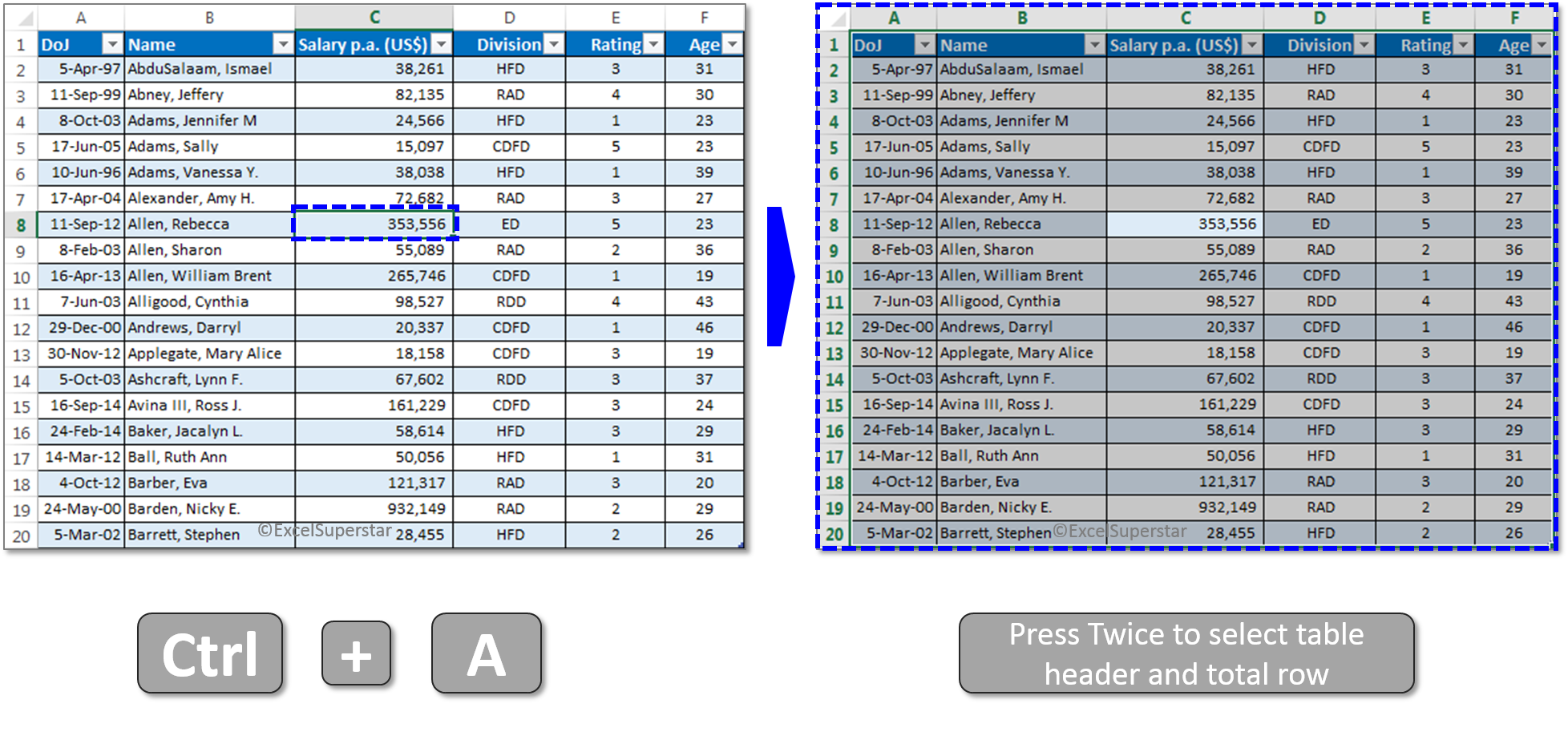
1st way: Use the Shortcut Key
1. Activate the table by clicking anywhere in the table.
2. Use the shortcut Ctrl + A to select the entire data in the table.
3. Press Ctrl + A again to select the column header and the total row.
2nd Way: Using the mouse
1) Hover the mouse to the top left-hand corner of the table until the cursor turns into a small black diagonal arrow pointing down.
2) Left Click on the mouse to select the body of the table.
3) Left-click on the mouse for the second time to select the table header and the total row.

3rd Way: Using the mouse
1. Activate the Excel Table by clicking anywhere inside the table.
2. Hover the mouse to any edge of the table until it turns into the four-way directional arrow
3. Left Click on the mouse.

NOTE: In this way of selecting the entire table you don’t need to click the left mouse button twice. One-Click is enough to select the entire table including Column Header and total row.