When you have a large set of data and need to evaluate the data also you need to do extra analysis it becomes difficult to know where all the functions in the file are coming from. Formula Auditing helps you out with this problem. Formula Auditing in Excel helps you to know the relationship between formula and the cell.
Formula Auditing too is an in-built function in Excel as like the other functions in Excel. Formula Auditing will help to get the spreadsheet properly audited.
In the earlier version i.e. in the Excel 2003 version, the Formula Auditing toolbar can be seen by right-clicking on the toolbar. Formula Auditing is a powerful component in Excel. There are several ways through which you can carry out formula auditing in Excel. To see the list of ways for carrying out formula auditing: Go to the Formula Tab > Formula Auditing group you will see six different ways.
1. Trace Precedents
2. Trace Dependents Remove Arrow
3. Remove Arrow
4. Show Formula
5. Error Checking
6. Evaluate Formula
The different ways through which you can become a master of formula auditing are explained in detail below with the help of an example.
1. Trace Precedents – formula auditing
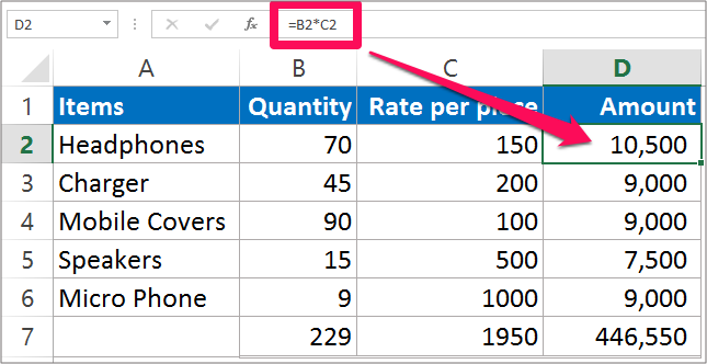
This function in Excel shows an arrow that indicates which cell affects the currently selected cells. When you activate the cell you see a blue hoax or arrow which shows the direction of the flow. To activate this function: Select the cell that contains the formula and Click on Trace Precedents in the Formula tab.
Precedent cells are those cells that affect the formula in the cell. Below you see an example that shows how you can trace precedents in Excel. If the Precedent is on a different sheet, a worksheet icon will appear at the beginning of the arrow.
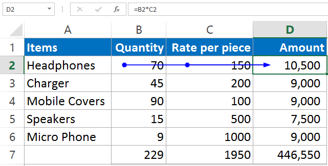
a. Click on the cell in the spreadsheet. Here we click on cell D2.
b. Go to the Formula tab > Click on Trace Precedents and The Result appears with a blue arrow.
2. Trace Dependents – formula auditing
This function in Excel shows arrows that indicate which cells are affected by the value of the currently selected cells. It shows arrows that indicate which cell is dependent on the selected cell.
If you have multiple formulas in the spreadsheet you can click on the Trace Dependents function, you can trace all the formulas in the spreadsheet. You can clearly know which cell was dependent to get the result.
To activate this function: Select the cell that contains the formula and Click on Trace Dependents in the Formula Auditing group under the Formula tab.
Dependents are those cells on which the formula is dependent. This function is of great use while we want to delete unnecessary information from the spreadsheet. Below you see an example that shows how you can trace dependents in Excel.
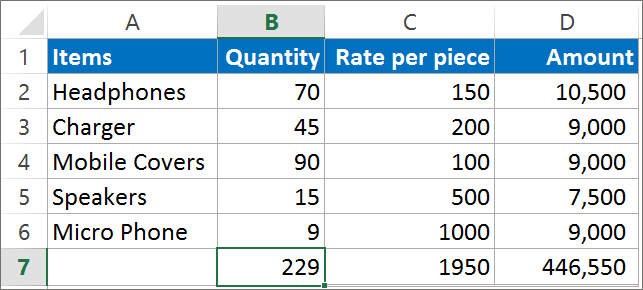
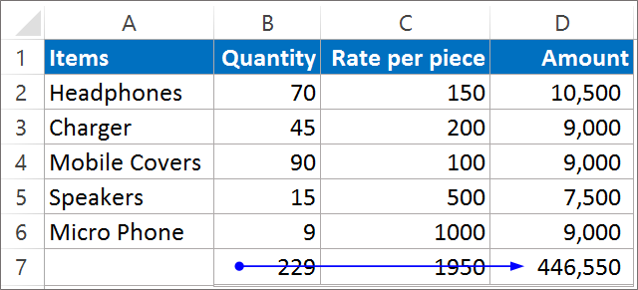
a. In our example, we have selected cell B7.
b. Go to the Formula tab > Click on Trace Dependents and The result will appear in the blue arrow.
3. Remove Arrow – formula auditing
Remove Arrow function can only take place once you have applied Trace Precedents or Trace dependents function in Excel. Remove arrow function is used to remove the lines that are shown. You see a drop-down arrow next to remove the arrow that shows three options:
a. Remove Trace Precedents Arrows: This option removes all the arrows that are related to trace precedents.
b. Remove Trace Dependents Arrows: This option removes all the arrows that are related to trace dependents.
c. Remove All Arrows: This option helps you to remove all the arrows that are both Precedent arrows and Dependent arrows.
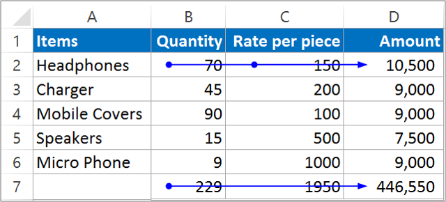
Here we have arrows that show Trace Precedents as well as Trace Dependents.
To remove the arrow you need to execute the following steps:
Go to the formula tab > in the formula auditing group > Click on Remove Arrow and As you click on any of the options you will see that all the arrows from the worksheet have disappeared.
4. Show Formulas – formula auditing
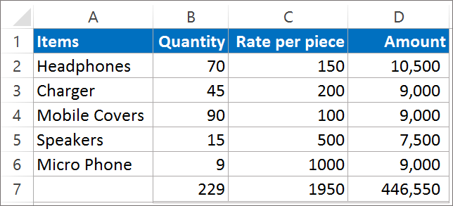
Excel shows the result of the formula and not the formula. It is the default setting to show the result instead of the formula. But, you have an option to view the formula instead of the result.
This function is useful when you want to see all the formulas used in the spreadsheet at a glance. Instead of clicking on individual cells and looking into the formula bar for the formula used, all you can do it click on the Show Formula function.
Go to the Formula tab > Click on Show formula in the Formula Auditing group.
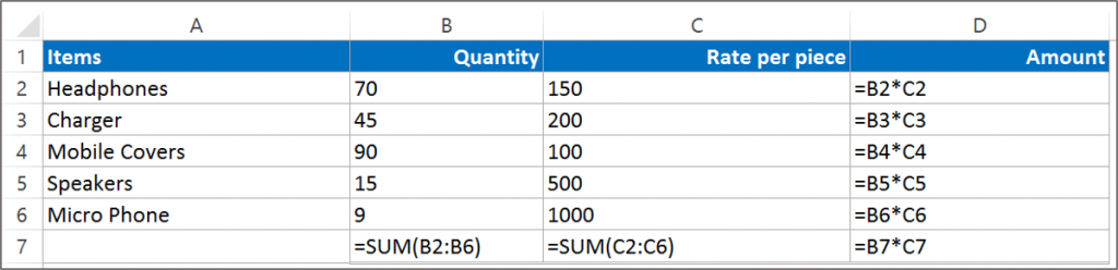
a. Click anywhere in the spreadsheet.
b.Go to the Formula Tab > Click on Show formula and The formula used in each cell of the spreadsheet will be displayed.
5. Error Checking – formula auditing
Error-checking by default is enabled in our Excel file. When you are not sure why the error has occurred in the formula you can do so by applying error checking. It is a good technique to use Error-checking once your spreadsheet is ready.
Error Checking is a formula auditing function that is available in the Formula tab under the group head Formula Auditing. As you click on the function Error Checking dialog box will open that will guide you to do what next.
Error checking checks for the common error that appear while using the formula. The drop-down menu also shows you an option to trace the error. The trace error option will help you to trace the cells which are linked.
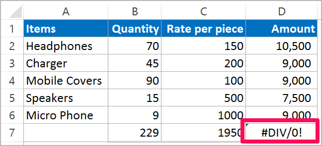
a. Click anywhere in the spreadsheet to activate the spreadsheet.
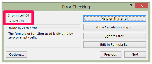
b. You see an error in the cell D7 of the spreadsheet.
c. Go to the Formula tab > Click on Error Checking and Error checking dialog box appear that shows where is the error in the spreadsheet and what is the error about.
d. Correct the error and you will the correct answer.
6. Evaluate Formula – formula auditing
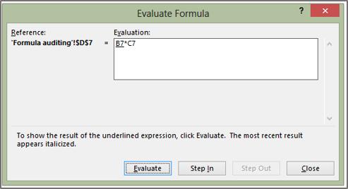
Evaluate Formula is used to debug a complex formula, evaluating each part of the formula individually. Stepping through the formula part by part can help you verify its calculation correctly. Clicking on Evaluate Formula will open an Evaluate Formula dialog box where the formula will be displayed in the evaluation box.
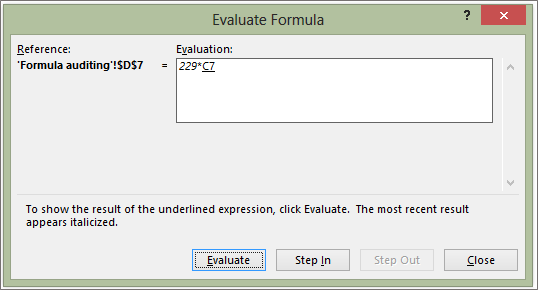
Click on the Evaluate button several times the formula gets evaluated. The underlined part of the formula will be executed next.
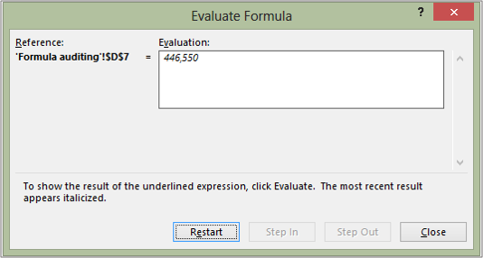
After Pressing Evaluate several times. You might see the Restart button at the place of the Evaluate button. This means that the evaluation is complete.
a. Click on any cell in the spreadsheet and click on the Evaluate formula in the formula tab. and In the Evaluate Formula dialog box, you see the formula in the Evaluation box. The underlined portion in the evaluation box is the part of the formula we are evaluating.
b. Click on Evaluate, you will see the other part of the formula that is being evaluated next.
c. Continue with the evaluate option until you find the Restart option.
d. This means that your evaluation is completed.