
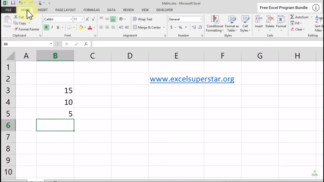
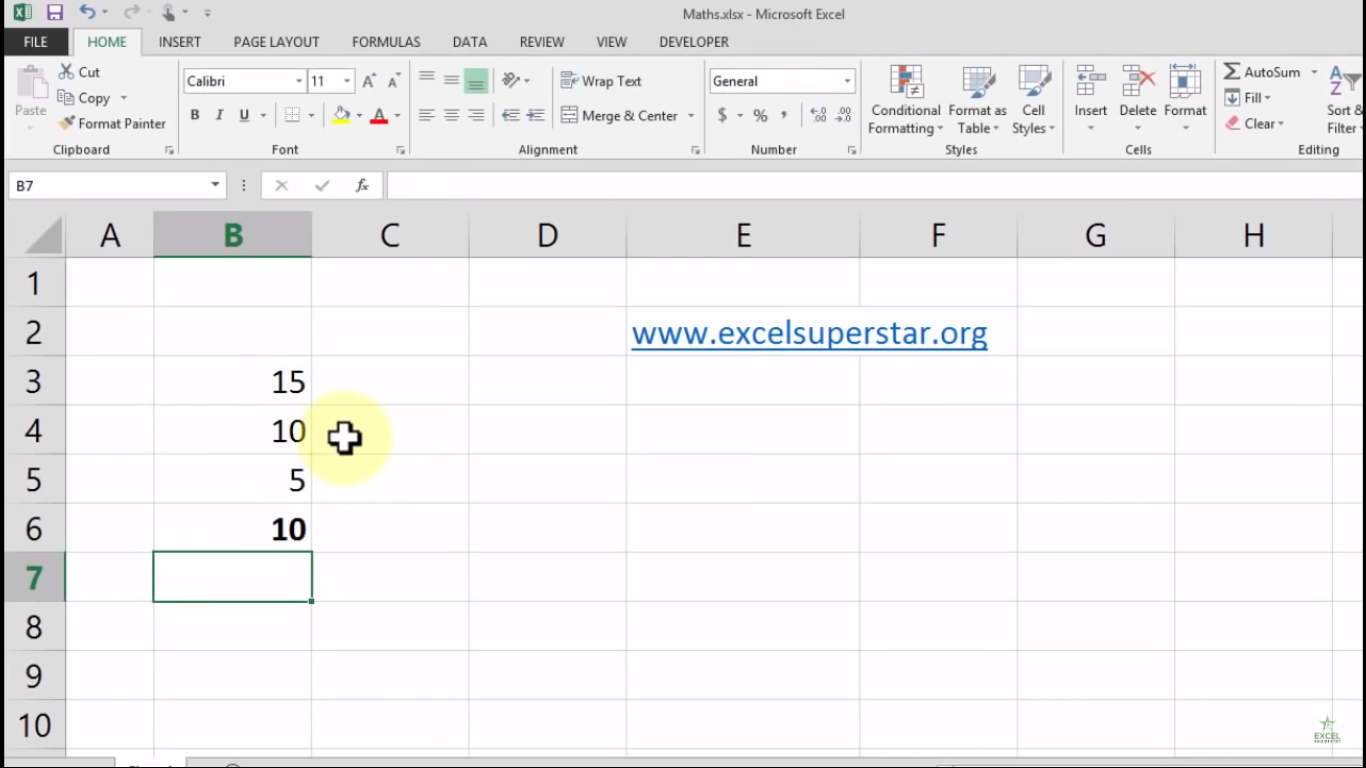
There is a column which consists of 3 numbers 15, 10, and 5. Now we want to calculate all 3 numbers in order to get the Average. So to calculate the average we have 2 methods given below:
Method 1:
1. Go to Home Tab

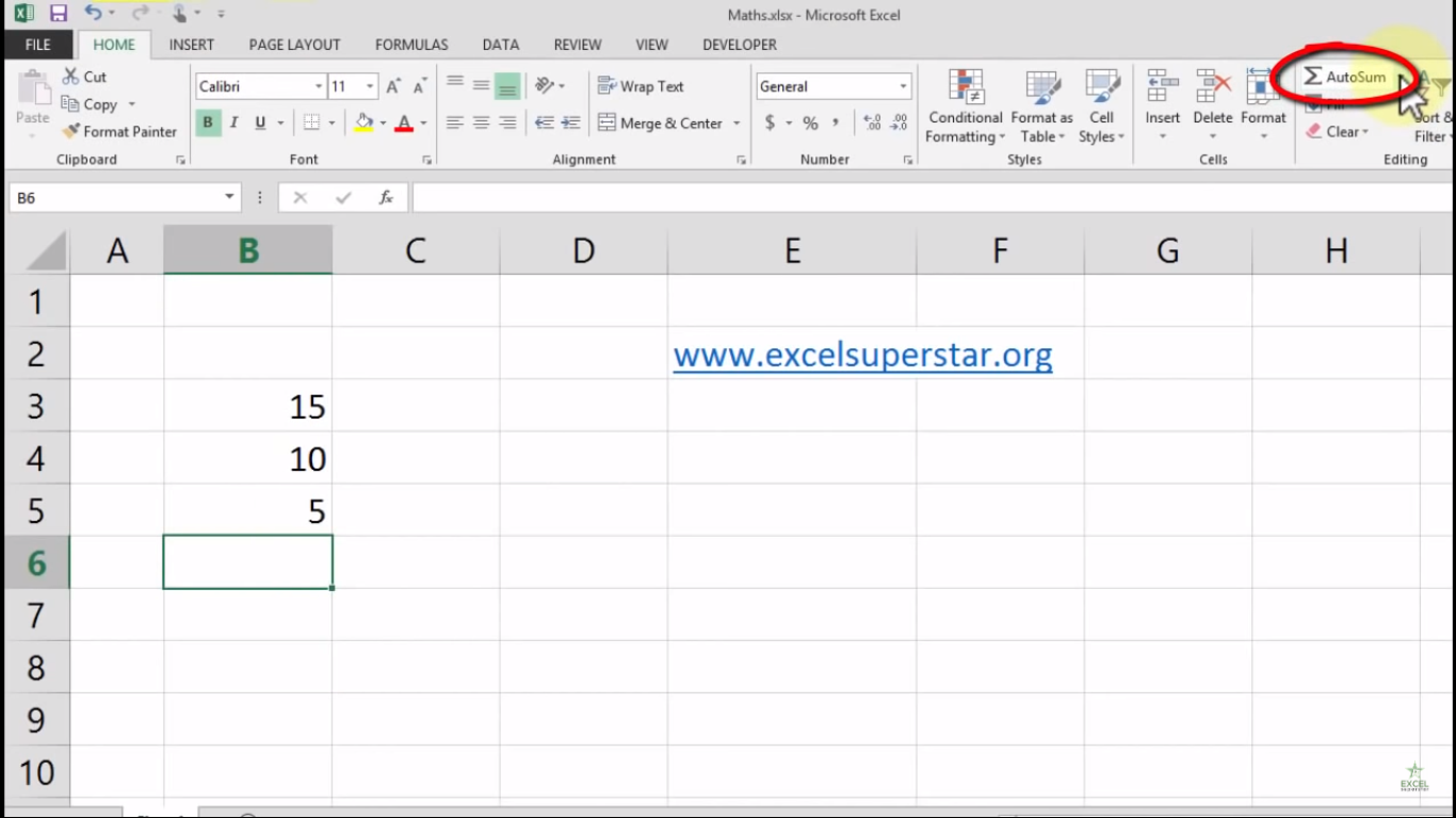
2. Click on AutoSum Dropdown
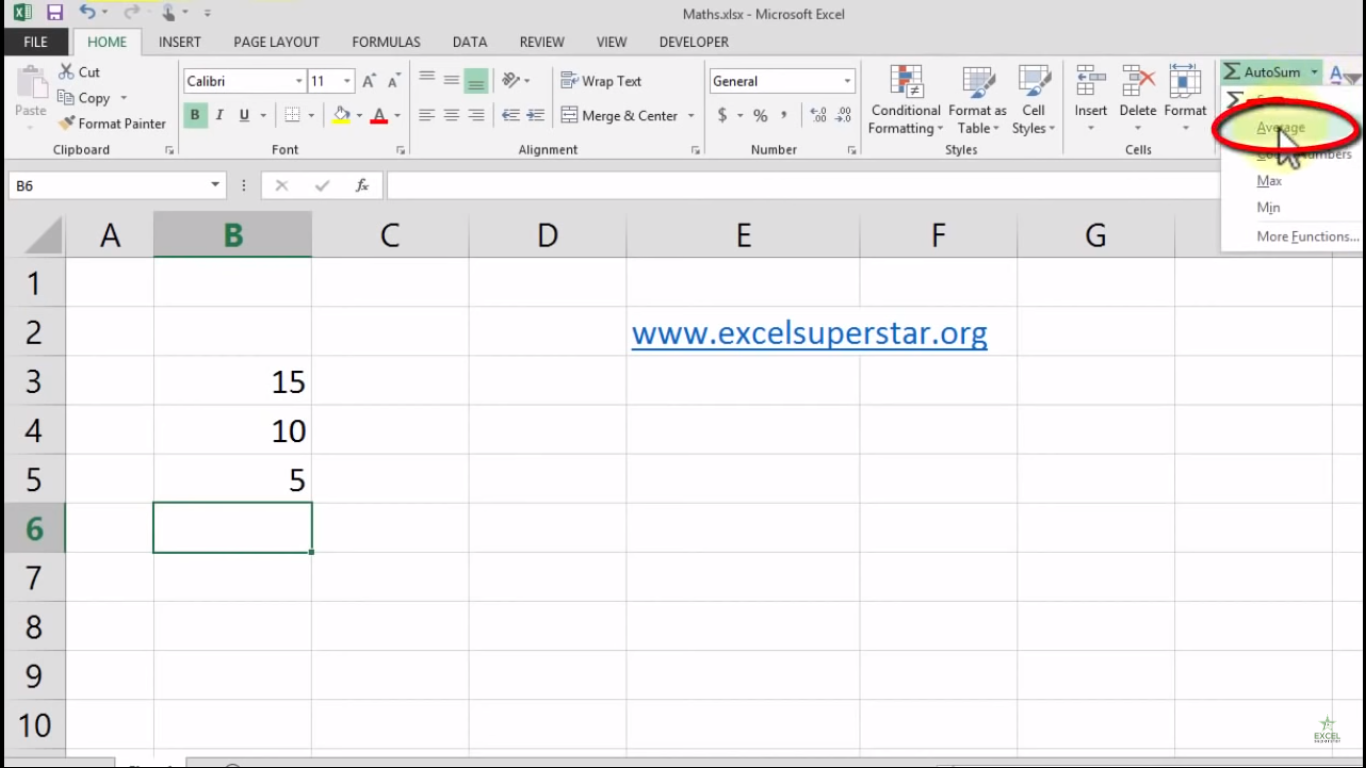
3. Select the Average Formula
4. You will see the Average Formula
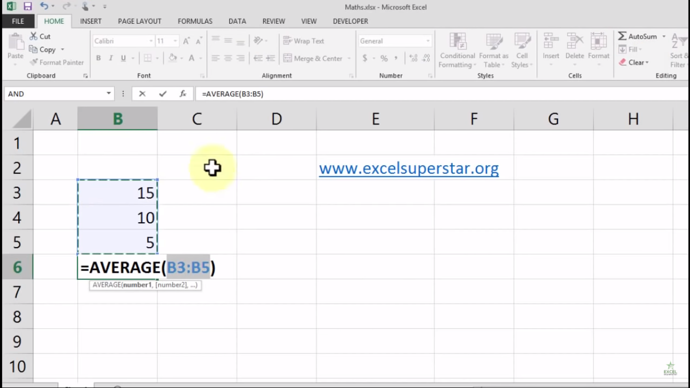
5. Press Enter and you will get your average answer as 10
Method 2:
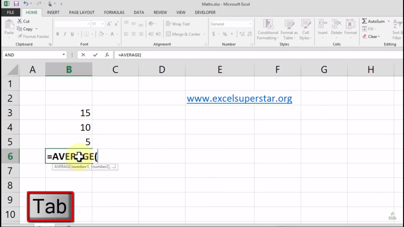
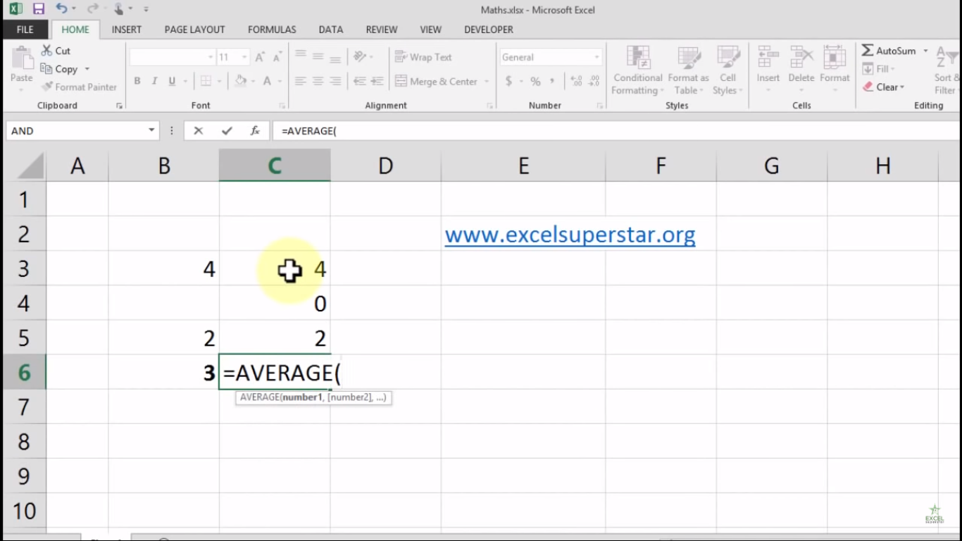
1. Write =ave and select the average formula from the dropdown by pressing the Tab key
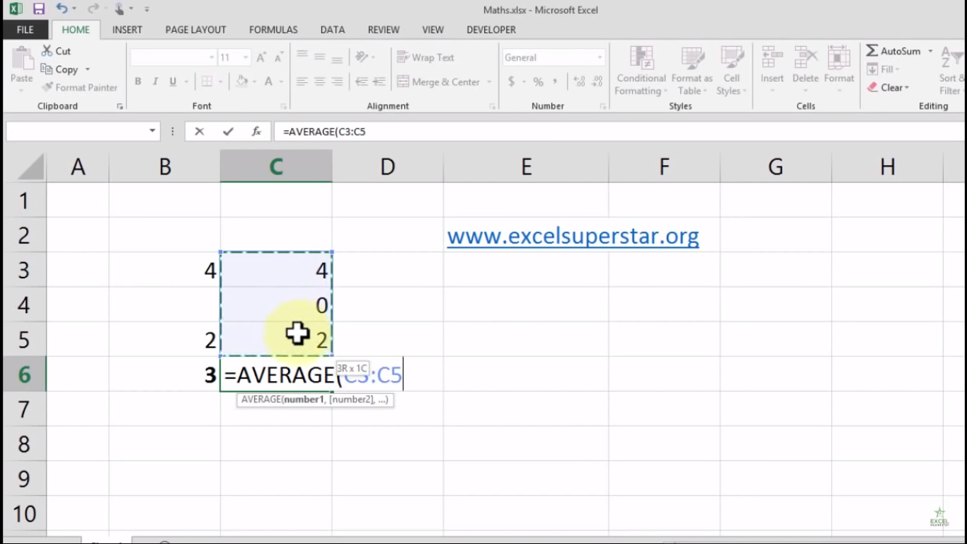
2. Select the entire range and close the bracket
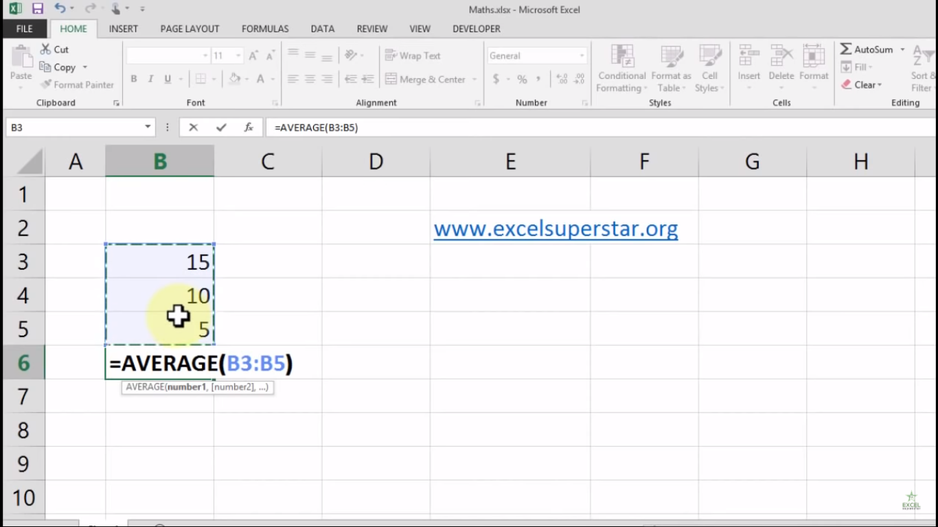
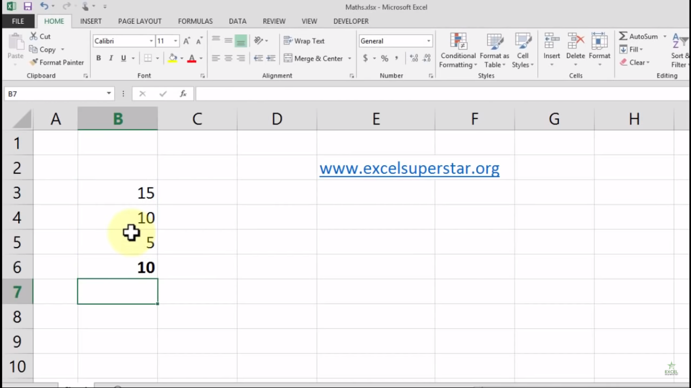
3. Press Enter and you will get your average answer as 10
Now suppose if you have two data
1. First Data
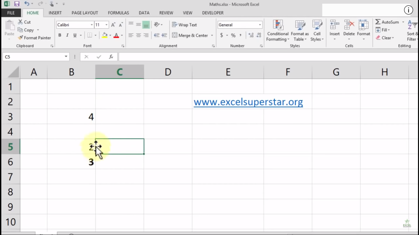
In the first data you have a blank cell and want to calculate the average of the data. So to calculate the average just follow the steps given below:
1. Write =ave and select the average formula from the dropdown by pressing the Tab key
2. Select the entire range and close the bracket
3. Press Enter and you will get your average answer as 3
2. Second Data
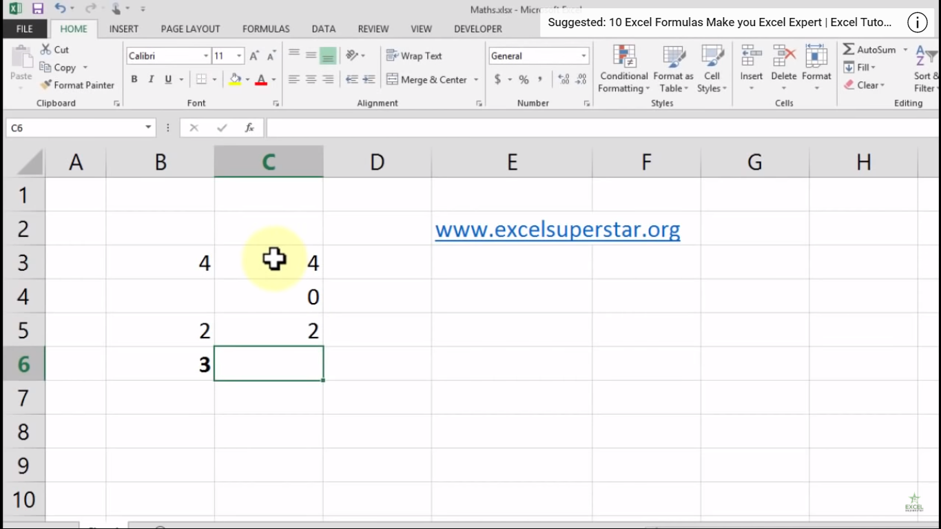
In the second data you have 0 in your data and want to calculate the data’s average. So to calculate the average just follow the steps given below:
1. Write =ave and select the average formula from the dropdown by pressing the Tab key
2. Select the entire range and close the bracket
3. Press Enter
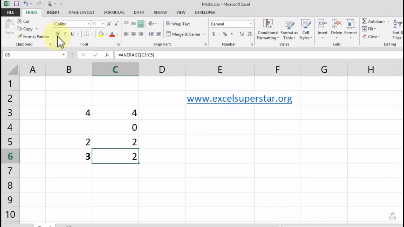
Note – Average Formula does not count the blank cells while calculating the Average but if you have 0 in your data then Average Formula counts 0 to calculate it.
4. Excel will calculate the average from the given data